Bayesian A/B Testing: Probability & Stopping Rules for Product Teams

Analyst comparing Bayesian experiment outcomes

Bayesian A/B testing tells you the probability that version B beats version A, plus a full distribution of how much better it might be. When you run one, monitor the posterior probability continuously, but only stop based on a decision rule you set before the test started, typically an expected-loss threshold or a calibrated Bayes-factor cutoff. The rest of this guide covers priors, models, stopping rules, and how to build this into a real workflow.

TL;DR:

Bayesian A/B testing updates beliefs using priors and data likelihood, producing a full distribution of possible uplift rather than a simple significance result.

The method allows continuous monitoring without inflating error rates when paired with a formal stopping rule like expected loss or Bayes-factor thresholds.

Priors should be checked via prior predictive simulations and sensitivity analysis, with empirical Bayes options available for leveraging past experiment data.

The Beta-Binomial model is ideal for binary conversion metrics, while continuous data like revenue require Normal or Gamma models for accurate analysis.

Proper validation, pre-declaring decision rules, and simulation calibration are essential steps before trusting Bayesian test results in production.

What Bayesian A/B Testing Actually Measures
How Bayesian Differs From Frequentist Testing
Choosing And Validating Your Priors
Matching The Model To The Metric
Reading The Posterior: P(B>A) And Credible Intervals
Setting Stopping Rules Before You Peek
Planning Sample Size Without Frequentist Power Formulas
Pooling Across Experiments With Hierarchical And Empirical Bayes
Building It: Tools, Code Paths, And Production Notes
A Short Checklist Before You Trust Your Results
Why Gostellar Approaches Experimentation This Way
The Practical Verdict On Bayesian Testing
Run Your Bayesian Tests Without The Setup Overhead
Sources

What Bayesian A/B Testing Actually Measures

Every Bayesian test starts with a prior, your belief about conversion rates or revenue per visitor before you see any new data. That belief gets combined with the likelihood, the pattern actual visitor data shows, to produce a posterior: an updated, evidence-weighted estimate of how each variant performs. This is different from asking "is this result statistically significant?" You're asking "given everything I know, what's the probability B is better, and by how much?"

That second half, the "by how much," is where Bayesian methods pull ahead of a simple significance test. The output isn't a single yes/no. It's a full distribution over possible uplift values, from which you compute P(B>A), the probability that variant B genuinely outperforms A.

Picture a landing page test where A converts 1,000 visitors and B converts 1,050 out of similar traffic. A frequentist test might report a p-value hovering near 0.06, technically not significant. That's a materially different conversation with a product manager than "not significant, kill it."

Key elements that make this system work together:

Prior: your starting assumption, which can be nearly flat (uninformative) or shaped by past experiments.
Likelihood: the probability of observing your actual data given a particular conversion rate.
Posterior: prior and likelihood combined, updated automatically as new data arrives.
Credible interval: the range where the true effect likely falls, given the posterior.

Nothing here demands a fixed sample size before you can look at results. That's the operational advantage worth understanding next.

How Bayesian Differs From Frequentist Testing

A frequentist test asks: "If there were truly no difference between A and B, how surprising is this data?" A Bayesian test asks: "Given this data, what's the probability B actually beats A, and by how much?" Those are fundamentally different questions, and they produce different guidance for how you should behave while a test runs.

Frequentist tests assume a fixed sample size decided in advance. Peek at results early and stop when you like what you see, and your real false-positive rate balloons well past the 5% you thought you were protecting. Bayesian methods handle continuous monitoring far more gracefully. Research on Bayesian methods for safe sequential testing shows that with a properly formalized stopping rule, teams can check results daily and stop early without inflating error rates the way naive peeking does under frequentist assumptions.

That said, "Bayesian" doesn't mean "immune to peeking problems." Stopping the moment P(B>A) crosses 95% with no other rule still introduces bias. The protection comes from pairing continuous monitoring with a formal decision rule, not from the framework alone.

Where each approach tends to fit best:

Frequentist: regulatory or scientific contexts where a pre-registered, fixed design is required.
Bayesian: marketing and product experiments where speed, interpretability, and continuous decision-making matter more than a rigid protocol.
Bayesian: situations where stakeholders want a probability and a dollar-value uplift range, not a binary reject/fail-to-reject outcome.

A deeper walk through the Bayesian versus frequentist testing tradeoffs covers scenarios where each method genuinely outperforms the other.

Choosing And Validating Your Priors

A prior is a starting guess, and how tight or loose that guess is changes how fast your posterior moves. A weak Beta(1,1) prior treats every conversion rate between 0% and 100% as equally plausible before you see data, which is honest but slow to update. A stronger prior, say Beta(50,950) reflecting a historical 5% baseline conversion rate, pulls early results toward that baseline until enough new data overwhelms it.

Neither choice is automatically correct. A weak prior wastes early data fighting against noise. A prior that's too concentrated on an unrealistic value can produce misleading posteriors even with substantial sample sizes, an issue the PyMC example gallery on Bayesian A/B testing illustrates directly through prior predictive checks.

A prior predictive check works by simulating fake data purely from your prior, before touching real numbers, and asking whether the simulated outcomes look plausible. Run a sensitivity analysis alongside it: refit the model with a few reasonable alternative priors and check whether your conclusion about P(B>A) shifts meaningfully. If it does, you need more data before trusting the result.

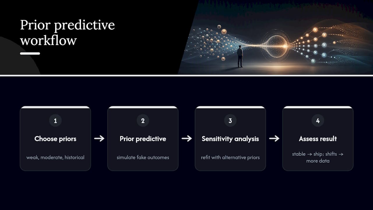
Prior predictive check and sensitivity workflow

Empirical Bayes takes this further by estimating the prior itself from a corpus of your own past experiments rather than guessing. Teams running dozens of tests a year can fit a program-level prior from historical win rates and effect sizes, which produces calibrated shrinkage: extreme early results get pulled toward realistic values automatically.

Pro Tip: Before your first live Bayesian test, run a prior predictive check on paper with three prior candidates: weak, moderately informative, and one built from last year's average conversion rate. If all three lead to the same shipping decision, your prior choice barely matters. If they disagree, that disagreement is telling you something.

Matching The Model To The Metric

Most conversion metrics, click-through, signup, checkout completion, are binary: a visitor either converts or doesn't. That maps cleanly onto the Beta-Binomial model, where a Beta prior combined with binomial trial data produces a Beta posterior in closed form. No simulation required, no iterative fitting. This is the workhorse model behind most Bayesian A/B testing tools for exactly that reason.

Revenue and other continuous metrics need different tools. Average order value or time-on-page rarely follow a binomial pattern, so a Normal-Normal model (assuming roughly symmetric, bell-shaped data) or a Gamma model (better suited to skewed, always-positive values like spend) fits more naturally. For metrics like revenue per visitor, many teams model two components separately, the probability of any purchase and the value given a purchase, then multiply the resulting distributions together to get expected revenue per visitor.

A few practical guidelines for model selection:

Use Beta-Binomial for any yes/no conversion event; it's fast, closed-form, and well understood.
Use Normal-Normal for roughly symmetric continuous metrics like session duration.
Use Gamma or log-normal variants for skewed, positive-only metrics like order value or revenue.
Reach for hierarchical models when you're running the same metric across many segments, pages, or markets and want them to share statistical strength.

Hierarchical models matter most when individual segments have thin data on their own, a new geography, a small traffic page, a niche user segment, but belong to a broader family of related tests where pooling improves estimates without erasing real differences between segments.

Reading The Posterior: P(B>A) And Credible Intervals

Two computational paths get you to a usable posterior. Closed-form Beta updates work when your model is a simple Beta-Binomial: you literally add successes and failures to the prior's parameters and read off the new Beta distribution directly, no simulation needed. Monte Carlo sampling becomes necessary once your model gets more complex, hierarchical structures, custom priors, multiple metrics combined, where no clean formula exists.

Here's the practical sequence for turning a posterior into a business answer:

Draw samples from each variant's posterior, typically tens of thousands of draws using a Beta-Binomial Monte Carlo approach or a probabilistic programming tool.
Subtract the paired draws (B minus A) to build the full distribution of the difference, not just its average.
Calculate P(B>A) as the fraction of those difference draws that land above zero.
Compute the credible interval, often the 95% highest density interval (HDI), which captures the most probable range for the true uplift.
Check the interval's width. A narrow HDI entirely above zero supports confident shipping. A wide HDI straddling zero means you genuinely don't know yet, regardless of what P(B>A) alone suggests.

That last step trips people up constantly. The probability tells you direction; the interval tells you how much you actually know about magnitude. Both numbers matter, and reporting only one to a marketing team is how good-sounding tests turn into bad launches.

Setting Stopping Rules Before You Peek

Decide your stopping rule before the test starts, not while you're watching the dashboard. The strongest teams pick one of two approaches: an expected-loss threshold or Bayes-factor stopping, and they commit to it in writing before traffic hits either variant.

Expected loss measures the average cost of choosing wrong. If you pick B but A was actually better, expected loss quantifies how much that mistake would cost in your actual business metric, revenue per visitor, signups, whatever you're optimizing. You set a threshold, L*, calibrated to what your business considers an acceptable risk, and you stop only when expected loss for your chosen variant drops below that threshold. A $0.02 threshold on revenue per visitor might be appropriate for a low-traffic test; a $0.002 threshold might suit a high-stakes checkout flow.

Bayes-factor stopping works differently. Rather than measuring cost, it tracks the strength of evidence for one hypothesis over another as data accumulates, and it's built specifically to preserve error-rate guarantees even when you check results every single day. Research on Bayesian inference procedures for A/B testing organizes this into a tiered framework, showing that Bayes-factor stopping bounds false-positive rates under continuous monitoring and comes close to minimizing expected loss for many common business cost structures.

Bayes-factor stopping is near-optimal across a broad class of cost functions, meaning teams don't have to choose between rigor and speed nearly as often as the frequentist framework implied.

Without a loss calibration or Bayes-factor structure behind it, that threshold has no formal connection to your actual error rate. Continuous monitoring against it can inflate practical mistakes well beyond what the number implies.

Before rolling any of this into production, run simulation-based calibration: generate thousands of fake experiments under your chosen prior and stopping rule, check how often the rule leads to correct decisions, and adjust before you bet real traffic on it.

Common stopping approaches, ranked by rigor:

Raw P(B>A) threshold: fast, but no formal error guarantee.
Expected-loss threshold: ties stopping directly to business cost.
Bayes-factor stopping: preserves error-rate bounds under continuous monitoring.

Planning Sample Size Without Frequentist Power Formulas

Bayesian planning doesn't use the classic power calculation (the probability of detecting a true effect at a fixed sample size). Instead, it uses assurance, the probability your chosen stopping rule leads to the correct decision, averaged across a realistic range of possible true effect sizes rather than one assumed value.

The output tells you, for a given daily traffic level, how many days it typically takes to reach a confident call, and how often that call turns out right.

This matters because fixed power calculations assume you already know the true effect size, which defeats the purpose of testing in the first place. Assurance instead builds in your genuine uncertainty about that effect.

Practical planning steps for common traffic situations:

Low-traffic pages (under 1,000 visitors weekly): expect longer runtimes; lean on informative or empirical Bayes priors to compensate for sparse data.
Medium-traffic pages (1,000 to 10,000 weekly): a two to three week simulation-calibrated run is typical for moderate effect sizes.
High-traffic pages (10,000-plus weekly): assurance simulations often show confident calls within days, but resist stopping before your pre-declared rule triggers.
Use a Bayesian A/B test calculator to sanity-check rough Beta-Binomial scenarios before committing engineering time to a full simulation.

Pooling Across Experiments With Hierarchical And Empirical Bayes

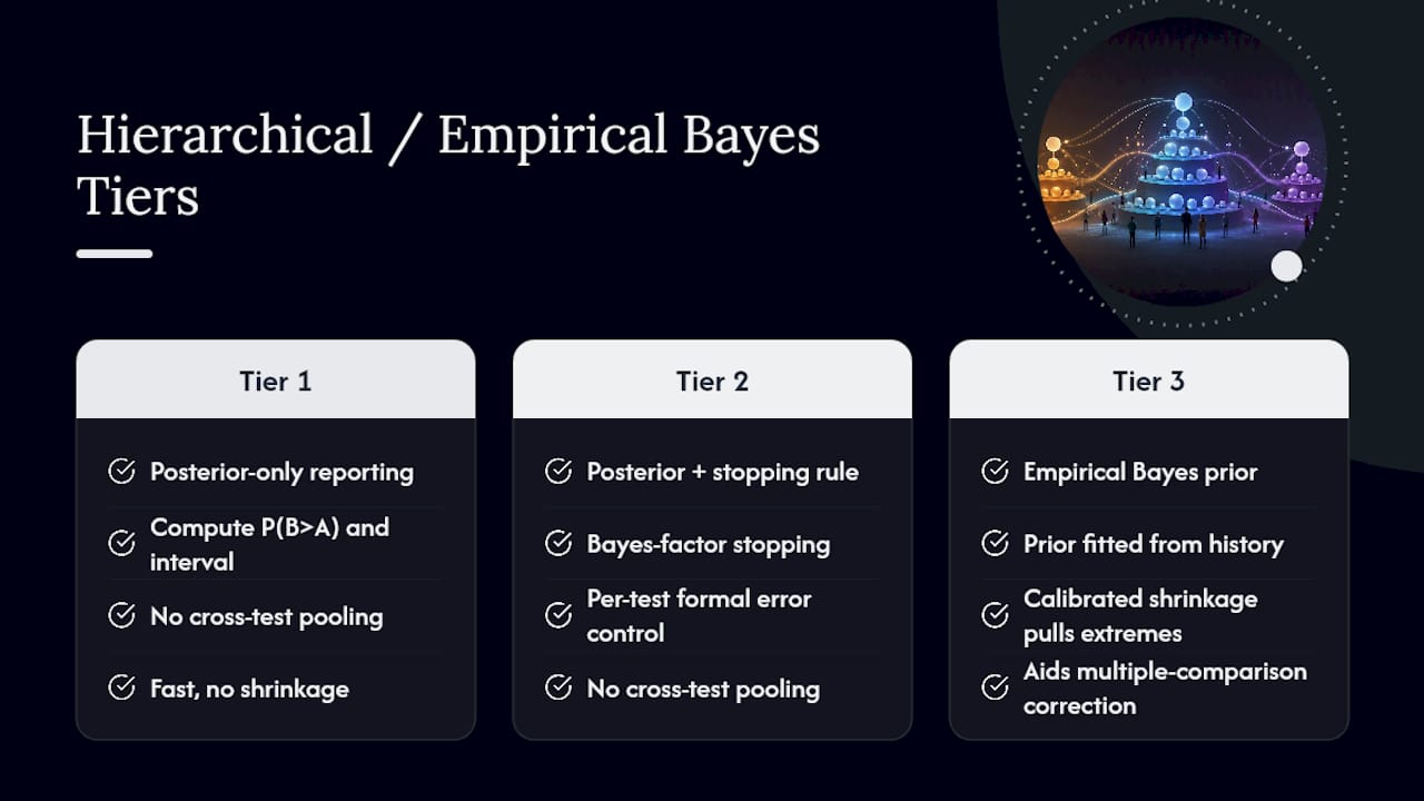
Programs running many tests a year benefit from a structure that treats each experiment not as an isolated event but as one draw from a family of related experiments. That's the logic behind hierarchical and empirical Bayes approaches, and it maps onto three practical tiers.

Tier 1 is posterior-only reporting: compute P(B>A) and an interval per test, no cross-test pooling. Tier 2 adds Bayes-factor stopping for formal error control within each individual test. Tier 3 adds an empirical Bayes prior fitted from your own historical corpus of past experiments, which delivers calibrated shrinkage (pulling extreme early estimates toward realistic values) and something close to automatic correction for multiple comparisons across metrics, according to the Bayesian inference procedures overview.

The power gain from pooling can be substantial. Research on scalable Bayesian A/B testing found hierarchical estimation materially increases statistical power in multivariate designs by letting related tests borrow strength from each other, which speeds up confident launches without loosening error control.

Pooling isn't free of risk. It assumes your past tests are exchangeable with your current one, similar traffic sources, similar user intent, similar time period. Program drift (your audience shifting over a year), seasonality, or mixing wildly different metrics into one pooled prior all break that assumption and can quietly bias results toward a stale baseline.

Pro Tip: Before trusting a Tier 3 empirical Bayes prior, check whether your historical corpus spans at least one full seasonal cycle and excludes any period where traffic sources changed dramatically. A prior built on six months of paid traffic won't generalize to organic.

Pooling Across Experiments With Hierarchical And Empirical Bayes — overview diagram

Building It: Tools, Code Paths, And Production Notes

Two implementation paths cover almost every real use case. The first is closed-form Beta-Binomial computation: fast, requires no simulation library, and handles the vast majority of conversion-rate tests. Lightweight packages like the benovamurat Bayesian A/B testing toolkit implement exactly this, bundling Beta-Binomial posteriors, Monte Carlo P(B>A) calculation, expected-loss decision rules, and HDI computation into a small, auditable codebase.

The second path is full probabilistic modeling with tools like PyMC or Stan, warranted when you need hierarchical structure, custom likelihoods, or multiple metrics modeled jointly. The PyMC example gallery walks through Beta-Binomial setups, prior predictive checks, and multi-variant extensions with working notebooks worth adapting directly. For hypothesis-style Bayes-factor computation with formal prior elicitation options, the abtest R package documents a production-tested alternative.

Choosing between the two paths:

Pick closed-form Beta-Binomial for single-metric conversion tests where speed and simplicity matter more than flexibility.
Pick PyMC or Stan when you need hierarchical pooling, custom revenue models, or several metrics evaluated jointly.
Use the abtest package when Bayes-factor hypothesis testing with formal null-evidence reporting fits your reporting requirements better than a pure probability statement.

Implementation path	Best for	Setup effort
Closed-form Beta-Binomial	Single conversion metric, fast iteration	Low
PyMC / Stan hierarchical	Multiple segments, revenue models, pooling	Moderate to high
abtest (Bayes factor)	Formal null-evidence reporting, continuous monitoring	Moderate

Production reliability depends on habits that have nothing to do with the math: fix random seeds so results are reproducible, log every experiment's prior choice, stopping rule, and start/end date as metadata, and wire posterior calculations into your existing analytics pipeline and feature-flag system rather than running them as one-off scripts. An experiment lifecycle that automatically archives configuration alongside results saves painful reconstruction work six months later when someone asks why a test was shipped.

A Short Checklist Before You Trust Your Results

Most Bayesian A/B testing mistakes come from skipping a step that felt optional at the time. Run through this before calling any test:

Confirm your decision rule was set before you started monitoring, not chosen retroactively once results looked favorable.
Run a prior predictive check and at least one sensitivity analysis with an alternative prior.
Verify pooling assumptions if using hierarchical or empirical Bayes models; check for seasonality or traffic-source shifts in your historical corpus.
Log the experiment's full configuration: prior, model, stopping rule, and timeline, before results come in.
Keep guardrail metrics visible alongside your primary metric so a win on conversion doesn't mask a loss on revenue or retention.
Re-run simulation-based calibration periodically, especially after changing traffic sources or audience mix.

Skipping step one is the single most common failure mode: teams that monitor P(B>A) daily with no pre-declared threshold end up making the stopping decision emotionally, the moment the number looks good, which reintroduces exactly the bias Bayesian methods were supposed to avoid.

Why Gostellar Approaches Experimentation This Way

Bayesian methods reward teams that can iterate fast and check results often without breaking their error guarantees, and that's precisely the operational environment Gostellar's tooling is built around. A lightweight 5.4KB script means real-time posterior monitoring doesn't come at the cost of page speed, and the no-code visual editor lets marketers launch variants without waiting on engineering, which matters when your stopping rule depends on getting to a usable sample quickly.

Real-time analytics dashboards give data scientists and product managers the same live view of conversion data that a Beta-Binomial posterior needs, updated continuously rather than batched. For teams applying the sequential monitoring approach discussed throughout this piece, that immediacy is what makes calibrated, pre-declared stopping rules practical instead of theoretical. Pairing that infrastructure with a Bayesian A/B test calculator closes the loop between conceptual understanding and daily decision-making.

The Practical Verdict On Bayesian Testing

The conventional pitch for Bayesian A/B testing oversells "you can peek anytime" and undersells the discipline it still demands. Peeking safely isn't automatic. It's earned by pre-declaring a real stopping rule, expected loss or Bayes-factor, and running simulation-based calibration before you trust that rule with production traffic. Skip that groundwork and you've just replaced one form of p-hacking with another that sounds more sophisticated.

What's genuinely underrated is the uplift distribution itself. Most teams fixate on P(B>A) crossing some threshold and ignore the width of the interval around it, which is often the more honest signal of whether you actually know anything yet.

Prioritize this in order: pick your decision rule first, validate your prior second, and only then start watching the dashboard. Empirical Bayes and hierarchical pooling are genuinely powerful, but they're a program-level upgrade for teams already running the fundamentals correctly, not a starting point.

— Juan

Run Your Bayesian Tests Without The Setup Overhead

Everything in this guide, priors, posteriors, expected-loss thresholds, still requires a testing platform that can actually capture clean data fast enough to make sequential monitoring worthwhile. A/B testing platforms typically offer no-code visual editors for launching variants without an engineering queue, dynamic keyword insertion for personalized landing page tests, and lightweight scripts designed to minimize page speed impact, along with handy conversion rate optimization tips to boost your test outcomes.

Gostellar

For marketers and product teams who want to apply the decision rules covered here without hand-rolling a Beta-Binomial script from scratch, start with the Bayesian A/B test calculator to model your next experiment's likely duration and uplift range. Businesses tracking a modest number of monthly users can explore available free tiers on A/B testing platforms to experience real-time goal tracking and posterior-style reporting on live tests.

Sources

The ArXiv overview of Bayesian inference procedures lays out the three-tier framework referenced throughout this guide and is the strongest single reference for understanding stopping-rule guarantees. The PMC article on sequential testing covers safe continuous monitoring in accessible terms. The J Stat Soft abtest paper documents a production R package for Bayes-factor testing. The PyMC example gallery offers runnable notebooks, and the benovamurat toolkit gives a lightweight Python starting point for teams building their own pipeline.

Try Stellar A/B Testing for Free!